PyTorch is one of the most used frameworks in the field of deep learning. We can use this library in every aspect and field data science and machine learning. We can also use it for reinforcement learning. In one of our articles, we have discussed reinforcement learning and the procedure that can be followed for building reinforcement learning models using TensorFlow in detail. In this article, we will discuss how we can build reinforcement learning models using PyTorch. The major points to be discussed in this article are listed below.
Table of contents
The CartPole problem Importing librariesDefining setupStoring memoryDeep Q network Algorithm Training of network
Let’s start with understanding the CartPole problem.
The CartPole problem
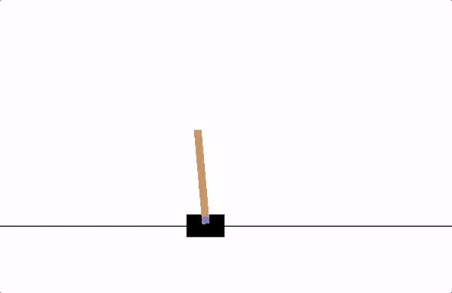
In this article, we are dealing with the CartPole problem. Where we will try to make an agent learn to decide whether to move the cart on the left side or right side so that the pole attached to the cart will be straight. We can see an example in the below image.
Internally, any action taken by an agent depends on the state of the environment, as the environment changes its state it returns a reward to the agent that decides the action of the agent at that state of the environment.
Here in this procedure, we will use +1 rewards at every timestep and if the cart moves more than a limit from the centre (here it is 2.4 units) or the pole will fall over too far, the environment will not return any reward to the agent. This is how if the agent is performing well then only it will work for a longer duration and get larger rewards.
Using the below lines of codes we can render the CartPole problem.
import gym
import numpy as np
import matplotlib.pyplot as plt
from IPython import display as ipythondisplay
from pyvirtualdisplay import Display
display = Display(visible=0, size=(400, 300))
display.start()
env = gym.make(“CartPole-v0”)
env.reset()
prev_screen = env.render(mode=’rgb_array’)
plt.imshow(prev_screen)
for i in range(50):
action = env.action_space.sample()
obs, reward, done, info = env.step(action)
screen = env.render(mode=’rgb_array’)
plt.imshow(screen)
ipythondisplay.clear_output(wait=True)
ipythondisplay.display(plt.gcf())
if done:
break
ipythondisplay.clear_output(wait=True)
env.close()
Output:
Since it’s a combination of different frames we can not post this here. Running the above codes will give you every state of the agent and also through the visualization we can say that the environment has some states like velocity and position. Let’s start our procedure by importing libraries.
Importing libraries
In this article, we will look at how we can use PyTorch for reinforcement learning. For this purpose, we are required to have a PyTorch and gym environment installed in our environment. The installation can be performed using the following lines of codes.
!pip install gym
!pip install pytorch
Since I am using google colab for this, I already have these libraries installed in the environment. The following libraries are required in our process.
import gym
import math
import random
import numpy as np
import matplotlib
import matplotlib.pyplot as plt
from collections import namedtuple, deque
from itertools import count
from PIL import Image
From PyTorch, we are required to call the following libraries.
import torch
import torch.nn as nn
import torch.optim as optim
import torch.nn.functional as F
import torchvision.transforms as T
Using the above packages we will define layers in our neural network and opitm module will help in model optimization and autograd module will help in automatic differentiation.
Defining setup
Using the below lines of code we are unwrapping the CartPole-v0, setting up the matplotlib for visualization, and starting the GPU for the environment.
env = gym.make(‘CartPole-v0’).unwrapped
is_ipython = ‘inline’ in matplotlib.get_backend()
if is_ipython:
from IPython import display
plt.ion()
device = torch.device(“cuda” if torch.cuda.is_available() else “cpu”)
Storing memory
Basic reinforcement learning requires replay memory for the training of the network. So in some kind of storage, we are required to store observations of the agent that can be used later. Using two classes we can store memory.
Transition = namedtuple(‘Transition’,
(‘state’, ‘action’, ‘next_state’, ‘reward’))
This class is named tuple, this tuple represents the single transition of our environment.
class ReplayMemory(object):
def __init__(self, capacity):
self.memory = deque([],maxlen=capacity)
def push(self, *args):
self.memory.append(Transition(*args))
def sample(self, batch_size):
return random.sample(self.memory, batch_size)
def __len__(self):
return len(self.memory)
The main motive of defining this class is to buffer the transition observed recently in a cyclic way. We also define samples in this class that will select a random batch of transitions for training.
Deep Q network Algorithm
As in the normal reinforcement learning procedure here also we aim to train an agent on the policy that can maximize the cumulative reward. Talking about the main idea behind Q-learning is to utilize such a function that can tell us what will be the return of any action.
Given any action regarding a state, we can maximize our rewards using a policy. In our network, we are going to use 5 convolutional layers from PyTorch which means our network is a convolutional neural network. We also have two outputs. In effect, our network will try to predict the expected return for each action given the current state.
class DQN(nn.Module):
def __init__(self, h, w, outputs):
super(DQN, self).__init__()
self.conv1 = nn.Conv2d(3, 16, kernel_size=5, stride=2)
self.bn1 = nn.BatchNorm2d(16)
self.conv2 = nn.Conv2d(16, 32, kernel_size=5, stride=2)
self.bn2 = nn.BatchNorm2d(32)
self.conv3 = nn.Conv2d(32, 32, kernel_size=5, stride=2)
self.bn3 = nn.BatchNorm2d(32)
def conv2d_size_out(size, kernel_size = 5, stride = 2):
return (size – (kernel_size – 1) – 1) // stride + 1
convw = conv2d_size_out(conv2d_size_out(conv2d_size_out(w)))
convh = conv2d_size_out(conv2d_size_out(conv2d_size_out(h)))
linear_input_size = convw * convh * 32
self.head = nn.Linear(linear_input_size, outputs)
Using the below lines of code we can call either one element to determine the next action during optimization.
def forward(self, x):
x = x.to(device)
x = F.relu(self.bn1(self.conv1(x)))
x = F.relu(self.bn2(self.conv2(x)))
x = F.relu(self.bn3(self.conv3(x)))
return self.head(x.view(x.size(0), -1))
Training of network
Using the below codes we can instantiate our model and its optimizer.
Defining parameters
BATCH_SIZE = 128
GAMMA = 0.999
EPS_START = 0.9
EPS_END = 0.05
EPS_DECAY = 200
TARGET_UPDATE = 10
Getting the screen size will help us to initialize layers correctly based on the shape returned from the gym environment and get the number of actions.
init_screen = get_screen()
_, _, screen_height, screen_width = init_screen.shape
n_actions = env.action_space.n
Defining policy net and target net and evaluation of target net
policy_net = DQN(screen_height, screen_width, n_actions).to(device)
target_net = DQN(screen_height, screen_width, n_actions).to(device)
target_net.load_state_dict(policy_net.state_dict())
target_net.eval()
Defining optimizer
optimizer = optim.RMSprop(policy_net.parameters())
memory = ReplayMemory(10000)
We can also define some utilities for showing off the results.
Select_action is a utility for selecting actions using the epsilon greedy policy. Plot_durations is a utility for plotting the duration of episodes. The resulting plot will contain the main training loop.
steps_done = 0
def select_action(state):
global steps_done
sample = random.random()
eps_threshold = EPS_END + (EPS_START – EPS_END) *
math.exp(-1. * steps_done / EPS_DECAY)
steps_done += 1
if sample > eps_threshold:
with torch.no_grad():
return policy_net(state).max(1)[1].view(1, 1)
else:
return torch.tensor([[random.randrange(n_actions)]], device=device, dtype=torch.long)
Plot duration
episode_durations = []
def plot_durations():
plt.figure(2)
plt.clf()
durations_t = torch.tensor(episode_durations, dtype=torch.float)
plt.title(‘Training…’)
plt.xlabel(‘Episode’)
plt.ylabel(‘Duration’)
plt.plot(durations_t.numpy())
if len(durations_t) >= 100:
means = durations_t.unfold(0, 100, 1).mean(1).view(-1)
means = torch.cat((torch.zeros(99), means))
plt.plot(means.numpy())
plt.pause(0.001)
if is_ipython:
display.clear_output(wait=True)
display.display(plt.gcf())
Training loop
After defining model and optimizer settings we can train our model.
def optimize_model():
if len(memory) < BATCH_SIZE:
return
transitions = memory.sample(BATCH_SIZE)
batch = Transition(*zip(*transitions))
non_final_mask = torch.tensor(tuple(map(lambda s: s is not None,
batch.next_state)), device=device, dtype=torch.bool)
non_final_next_states = torch.cat([s for s in batch.next_state
if s is not None])
state_batch = torch.cat(batch.state)
action_batch = torch.cat(batch.action)
reward_batch = torch.cat(batch.reward)
state_action_values = policy_net(state_batch).gather(1, action_batch)
next_state_values = torch.zeros(BATCH_SIZE, device=device)
next_state_values[non_final_mask] = target_net(non_final_next_states).max(1)[0].detach()
expected_state_action_values = (next_state_values * GAMMA) + reward_batch
criterion = nn.SmoothL1Loss()
loss = criterion(state_action_values, expected_state_action_values.unsqueeze(1))
optimizer.zero_grad()
loss.backward()
for param in policy_net.parameters():
param.grad.data.clamp_(-1, 1)
optimizer.step()
In the above codes, we first transpose the batch array of transition by computing the mask of non-final states. With this, we compute the expected q values, Huber loss and optimize the model. Using the below code we can visualize the main training loop. By resetting the state tensor we sample the action and execute it again, sample the next action and repeat the execution in the loop.
num_episodes = 50
for i_episode in range(num_episodes):
env.reset()
last_screen = get_screen()
current_screen = get_screen()
state = current_screen – last_screen
for t in count():
action = select_action(state)
_, reward, done, _ = env.step(action.item())
reward = torch.tensor([reward], device=device)
last_screen = current_screen
current_screen = get_screen()
if not done:
next_state = current_screen – last_screen
else:
next_state = None
memory.push(state, action, next_state, reward)
state = next_state
optimize_model()
if done:
episode_durations.append(t + 1)
plot_durations()
break
if i_episode % TARGET_UPDATE == 0:
target_net.load_state_dict(policy_net.state_dict())
print(‘Complete’)
env.render()
env.close()
plt.ioff()
plt.show()
Output:
We can see outputs in the runtime of the cell, for better results and optimization we can improve the number of episodes. The whole code for the procedure can be found here.
Final words
In this article, we have discussed the CartPole problem. For the environment, we used the Gym toolkit, and for solving it to an extent using an agent and reinforcement learning algorithm. We used the PyTorch framework to make them all work together.
References
Source: https://analyticsindiamag.com/a-guide-to-building-reinforcement-learning-models-in-pytorch/