Machine learning techniques are now very common in many spheres, and there is a growing popularity of these approaches in macroeconomic forecasting as well. Are these techniques really useful in the prediction of macroeconomic outcomes? Are they superior in performance compared to their traditional counterparts? We carry out a meta-analysis of the existing literature in order to answer these questions. Our analysis suggests that the answers to most of these questions are nuanced and conditional on a number of factors identified in the study.
Timely forecasts of key macroeconomic indicators, such as the gross domestic product (GDP) growth and inflation, are important for policymakers and market participants to gauge the health of the economy, form future expectations, and calibrate their actions. A central bank’s decision on whether to increase or decrease the monetary policy rate, a government’s expectations about the tax revenue it may obtain over the coming year, and decisions regarding investments—all require forming expectations about the inflation or GDP growth in a country that rests on a foundation of good forecasts.
In recent times, the use of machine learning (to be used interchangeably with the term ML in some places in this article) techniques is gaining popularity in various spheres.1 A limited but growing literature is also emerging that uses these new approaches for macroeconomic forecasts. While most of the research in this field is conducted in the United States (US) and other developed countries’ central banks, work has been undertaken recently in developing countries as well. However, a broad-based understanding about these approaches is yet to emerge. In this article, we attempt to contribute to a better understanding of these issues by undertaking a critical review of the relevant literature.
Machine learning is the “study of computer algorithms that improve automatically through experience” (Mitchell 1997). Statistical techniques for predicting a target variable, such as GDP growth or inflation, fall within the domain of “supervised learning.” This domain of statistics is primarily concerned with relating observations of a set of inputs or predictor variables represented by X, to a supervising output/response/target variable Y, through a function f—with some associated error ε (James et al 2013):
Y = f(X) + ε
For instance, if the past values of GDP or inflation (X) predict their future values (Y) reasonably well and are related through a linear function f, then using the same function, we can predict Y as more data on X become available. As Jung et al (2018) note, machine learning methods do not make assumptions about the functional form of f. Macroeconomic predictions using such methods are thus dependent on first estimating the shape or the “fit” of the function f, that is, how does it relate X and Y (on “training” or in-sample data), and checking whether this function does a good job of relating X and Y in the presence of previously unseen data (“test” or out-of-sample data).
In this article, we investigate the existing literature in macroeconomic forecasting on the advantages of machine learning approaches over traditional statistical techniques. We conduct a meta-analysis of the literature on forecasting the GDP growth and inflation using ML techniques. The aim is to understand whether ML techniques are better than their “standard” or non-ML counterparts in providing more accurate forecasts.
The structure of the article is as follows. The article begins with an introductory review of the ML techniques most commonly used in the existing literature. It then describes the data set constructed for our meta-analysis. After a discussion of the empirical results of the analysis, it concludes.
Machine Learning Techniques
ML methods most commonly used in the literature on forecasting growth and inflation can be broadly divided into three types: regularisation, tree-based, and neural networks. We introduce and describe each of these types below.
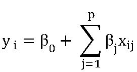
Regularisation: Parameter estimation used in most standard linear predic–tion methods follows the ordinary least squares (OLS) procedure. Take a standard linear regression as an example:
Estimating β using OLS requires minimising the sum of squared residuals (henceforth RSS):
This estimation works well in many situations. However, if the number of predictors is close to, or greater than, the number of observations, then estimation via OLS can lead to overfitting wherein the estimated parameters have low bias but high variance. This means that they might fit the relationship between the predictors and the response variable closely in the available sample (low bias) but are sensitive and prone to vary with the introduction of new observations—they will perform well in-sample but not out-of-sample (high variance), which is not good for a forecasting model.
However, with some modifications to the OLS procedure, some bias in parameter estimation can be introduced in order to reduce their variance, thereby improving their predictive performance. These modifications are provided by “regularisation” or “shrinking” techniques, such as Ridge regression, least absolute shrinkage and selection operator (LASSO), and elastic net.
Ridge regression: Ridge regression introduces a penalty in the estimation of parameters βj. This penalty is a simple addition to the OLS estimation procedure seen earlier:
The penalty , known as “shrinkage penalty,” is small when β1, β2, …, βj are close to zero. Therefore, minimising the RSS subject to the constraint imposed by the shrinkage penalty involves “shrinking” the coefficients towards zero. The tuning parameter (or “hyperparameter”) λ determines the relative importance of the penalty term. As is evident from the equation, if λ = 0, this term has no effect, and coefficients are estimated using the standard OLS procedure. As λ tends towards infinity, the effect of the penalty term grows, and coefficient estimates βj shrink towards zero. A different set of coefficient estimates are produced for each value of λ. Therefore, it is important to carefully select a value for the tuning parameter. This can be done using cross-validation where ridge regressions with varying shrinkage penalty values can be modelled to see where the bias-variance trade-off is minimised, leading to the lowest mean squared error (MSE). Broadly, cross-validation can be conducted by dividing the available data into k subsamples, parameterising the given model using k – 1 subsamples and testing its performance on the remaining subsample. This process is repeated until all subsamples have been used as the “test” sample. The MSE from different iterations of the model can be averaged to get an overall sense of the test performance of the model or gauge which value of the tuning parameter provides the lowest MSE.2
Least absolute shrinkage and selection operator: While ridge regressions regularise parameter estimates with high variance in order to improve their predictive ability, in data sets where the number of potential predictors is large, challenges still remain in interpreting models. For example, many predictors will have negligible coefficients, that is, they will not add value in terms of predictive content. In such situations, it can be difficult to parse which predictors are the most useful. The LASSO technique, much like ridge regression, shrinks the parameters towards zero to reduce their variance. However, it lets some parameters shrink exactly to zero when the tuning parameter λ is large enough so that those variables drop out of the model. This creates more sparse and more interpretable models with only those variables included that are relevant for predicting the response variable. This is achieved by changing the shrinkage penalty from :to
Like ridge regression, minimising the equation entails shrinking the parameter estimates towards zero. Due to the nature of the constraint set by the penalty term in LASSO, some variables are allowed to shrink to zero, given a large enough value of the tuning parameter. As before, cross-validation should be used to determine the optimum value of the tuning hyperparameter to balance the bias-variance trade-off.
Elastic net: A combination of LASSO and ridge regressions is the elastic net, which allow for a model to not be too dependent on the selection made by LASSO, yet allow for model interpretability by limiting the number of variables from a large predictor space. This is done by minimising the RSS subject to both ridge and LASSO penalties as shown below.
Source: Mahajan and Srinivasan (2020).
Here, we have two hyperparameters λ and α. λ, as before, ranges from 0 to infinity and increases the degree to which parameter estimates are shrunk. α, the new hyperparameter, determines the relative importance of the LASSO and ridge penalties. It ranges from 0 to 1. If α = 0, then the LASSO penalty drops out and we have a ridge regression. If α = 1, the ridge penalty drops out and we have a LASSO formulation. This combination allows for relatively stable coefficients (with low variance) in the presence of “fat” data (that is, with many possible predictors) and multicollinearity (Mahajan and Srinivasan 2020).
Tree-based methods: Tree-based methods involve partitioning the available predictor-space into a number of regions based on pre-specified rules and making a prediction for the response variable in each region. Since this partitioning can be graphically represented in a “decision-tree,” such methods are called “tree-based” methods or classification and regression trees (CART). Popular examples include Random Forests and its “bagged” or “boosted” implementations, which involve “growing” multiple trees. In order to understand them, however, we first need to understand how a single tree is grown.
First, the predictor-space composed of predictors X1, X2, …, Xj is divided into distinct, non-overlapping regions R1, R2, …, Rj. This is commonly done via recursive binary splitting. This entails taking all predictor observations as part of a single region at first. This predictor-space is then split on the basis of the predictor and a “cutpoint” that minimises the RSS across the two resulting regions. In other words, this partitioning rule searches across all predictors Rj to find an appropriate cutpoint s, such that we have two regions:
R1(j, s) = {X|Xj < s} and R2(j, s) = {X|Xj ≥ s}
where all values of Xj belonging to R1 are less than s, and the rest belong to R2. The goal behind this is to find the predictor Xj and cut-point s that minimise the RSS across all regions:
Here, y^R1 is the mean of the response variable for the training observations in region R1 and y^R2 is the mean of the response variable for observations in region R2.
This process is then repeated in the two regions R1 and R2 with the aim to find the predictor and cut-point that would minimise the overall RSS once more, thereby creating a third region. Subsequent regions are created in the same manner. This binary splitting continues until a stop-criterion is reached, that is, a maximum number of nodes or splits or a minimum number of observations in each region. Once the splitting concludes and we have regions R1, R2, …, Rj, we predict the value of the response variable in each region to be its mean,3 and a tree is thus grown.
With recursive binary splitting, it is easy to have a very high number of regions. Theoretically, it is possible to have a region for each training observation of the predictors, resulting in a perfectly fitted tree. However, overfitting leads to high variance and thereby poor out-of-sample predictions. The solution is “pruning” of trees. Pruning techniques complemented by appropriate cross-validation allow the user to select sub-trees that balance in-sample and out-of-sample prediction accuracy.4
Tree-based methods have many advantages. They are useful in modelling interactions between different predictors in a better manner than standard techniques, as the latter tend to create more regressors relative to data points (Mahajan and Srinivasan 2020). The relative importance of different predictors is also more intuitively understood in a decision-tree format. Nonetheless, while single trees can be intuitive to understand, their predictive performance can be poor. The solution to this problem is a group of models that grow multiple trees and are known as “bagging,” “random forests,” and “boosting,” respectively.
Growing multiple trees and aggregating the predictions that they provide improve upon the performance of the tree-based methods significantly. If all the predictors are available as candidates for splitting and the average prediction of multiple trees grown using bootstrapped samples is considered, it is called “bagging.”5 Bagging reduces the variance that accompanies a single tree. However, if the predictors are highly correlated, the reduction in variance will not be large since most trees will be grown in a similar order. Hence, growing multiple trees with different variables is useful in order to reduce prediction variance further. This objective is achieved by the group of models called “random forests.”
Random forests “decorrelate” the trees by modifying the bagging methodology. At each split in a tree, the learning algorithm is not allowed to consider all the available predictors. Using bootstrapping principles, multiple trees are then grown using multiple draws from the training sample. This is useful as it leads to different trees created out of different variables, which lowers the out-of-sample variance of the model.6
Random forests or bagging techniques develop multiple trees independently of each other and then average them. A third technique called boosting7 is slightly different from these two approaches as it grows trees sequentially. The advantage of this sequential process is that the residuals of the past trees are used to provide information that is used to grow newer trees. This allows the algorithm to learn “slowly” and improve the fit of each tree where its residuals are large. This sequential growing of trees lowers the forecasting error.
While techniques like random forests, bagging, and boosting can improve forecast accuracy over the predictions of single trees, it can be difficult to interpret the resulting models. For example, it is much easier to visually delineate important splits (variables) in a single tree, but an average of predictions over multiple trees cannot be as clearly visualised. Hence, tree-based methods that grow multiple trees improve predictions at the expense of interpretability. But, one can use prediction measures such as RSS and Gini indices to obtain summaries of the importance of each predictor, even if the relationship is not visually clear.
Artificial neural networks: Artificial neural networks, also known simply as neural networks, are a set of techniques that mimic biological decision-making processes using a set of inputs, analysing their relative importance, and using that information to determine an output. The earliest models of such nodal learning were known as “perceptrons” (Rosenblatt 1958) that used inputs (X1, X2, X3 … Xi) and their weights (w1, w2, w3 … wi) to determine the output as the weighted sums of the inputs. Neural networks however deal with more complex modelling objectives, and these are achieved by building sequential layers of multiple perceptrons, rather than a single one. These intricate network of perceptrons can be categorised into three parts, that is, an input layer, an output layer, and one or more hidden layers in between the input and output layers, each consisting of multiple nodes or “neurons.”
There are two more ways in which neural networks improve over simple perceptrons. The first is to introduce the possibility of non-linearity in the impact that weighted inputs have on the output. This works through the “activation function” that imposes a non-linear transformation on the weighted inputs before they provide information to the next neuron in the chain. Some of the commonly used non-linear functions used include sigmoid, tanh, and Rectified Linear Unit (ReLU) functions. The second way that a neural network improves its performance is by a process known as “backward propagation.” This is a feedback mechanism from the output error in any particular iteration (difference between the estimated output in that iteration and its actual value) back to the inputs, enabling an adjustment in their weights in the next iteration so that more and more accurate predictions become possible.
Figure 1 is a schematic representation of a single iteration of the process . There is an input layer that has two neurons (independent variables), a single hidden layer with three neurons and an output layer with a single neuron (target or dependent variable). The box highlights the first step in the process of running the model. The importance of each of these two input neurons (X1, X2) to the next neurons in the hidden layer (here 3, 4, or 5) is determined by their weights (w13, w14, w15) and (w23, w24, w25 ), respectively. Conversely, the information that can be received by any particular neuron in the hidden layer is a weighted summation of X1 and X2. Apart from the weighted inputs, another term that is added in this transformation is a “bias,” which is a constant and similar in concept and function to the intercept term in a linear regression. These are represented by (θ3, θ4, θ5) for neurons 3, 4, and 5, respectively. Finally, the chosen non-linear activation function is imposed on the weighted inputs (plus bias) before the results are transferred to the next neuron.
Next, we look at Figure 2. The box now highlights the next step in running the model. The transformations described earlier create derived variables for node 3, 4, and 5, respectively. The process in the first step is now repeated using these derived variables as inputs. This involves first assigning weights and biases to these inputs and then imposing the activation function on this transformation. The result is the output for the model for this round of iteration.8
Next, as described earlier, a process of “backward propagation” introduces circularity to the process in order to let the network learn which connections to emphasise and thus bring the final output closer to a desired value. This process uses a technique called “gradient descent” to efficiently find the direction and magnitude of change needed in the weights and biases used in all the steps of the second and subsequent iterations.9 This repeated iteration helps the model learn more and more about the data and provides an accurate prediction of the output or target variable.
While neural networks were initially designed to analyse cross-sectional data, they are increasingly being used in time series analysis by modifying the model to accommodate time dimensions as well. Deep neural networks (DNNs) build on this concept by having an increased number of hidden layers, leading to more complex transformations and functional relationships. However, DNNs alone cannot deal with the time series data adequately because the data are revealed to each node in the hidden layer simultaneously, as opposed to sequentially, to account for temporal dimensions. This is why using only DNNs in this iteration may not necessarily help to discern complex relationships that are shaped over time. Recurrent neural networks (RNNs), on the contrary, allow the incorporation of information sequentially, which is suitable for time series analysis. The structure of RNNs is the same as regular neural networks, with layers of neurons feeding-forward information. The basic difference is that RNNs create multiple “copies” of the same network, with each copy corresponding to each observation sequentially. The output from the first copy informs how the second one will determine its output, which in turn determines the third, the fourth, and so on. Needless to say, a drawback of such complicated versions of neural networks is that the computational power required to run them goes up substantially.
A Meta-analysis of the Literature
In this section, we carry out a meta-analysis of the literature that uses machine learning for macroeconomic forecasts. Our goal is to understand whether ML techniques tend to perform better than their non-ML counterparts in forecasting the GDP growth and inflation. Further, we attempt to find out the conditions under which they perform better: longer or shorter forecast horizons, in emerging or advanced economies, and so on.
Data: In order to conduct this meta-analysis, we assemble a data set of papers that utilises ML techniques in their forecasts of growth and inflation. Another criterion for the selection of papers was that their forecast period was more recent. While this criterion is inherently arbitrary, the aim is to ensure that our data are relevant since the global economy and inflation rules by central banks changed significantly close to and after 2000.10
In order to compile our data set, we traced the thread of citations that met our criteria, beginning with the most recently available papers. In other words, a 2021 paper meeting our criteria is included, its citations are searched to find more relevant papers, and this process is repeated for each of the papers identified through this process. Through this search process, we have been able to identify 16 papers that use at least one type of ML technique in forecasting either the GDP growth or inflation.11 Each of these papers also have 1-quarter and one-year-ahead forecasts that belong to the post-2000 period. Among the 16 papers, there is a relatively even split within four groupings: GDP growth in advanced economies, inflation in advanced economies, GDP growth in emerging economies, and inflation in emerging economies.
Within advanced economies, Jahn (2018), Biau and D’elia (2010), Jung et al (2018), and Richardson et al (2019) look at growth forecasting in the European Union countries, Japan, the US, and New Zealand; Jung et al is the only paper in the entire set that looks at both advanced and emerging economies (that is, Mexico, Philippines, and Vietnam). The papers in this set use univariate, multivariate, factor-based, regularisation, tree-based, and neural network methods on their samples. While Jahn (2018) uses regular neural networks, Jung et al (2018) use RNNs.
Teräsvirta et al (2005), Medeiros et al (2019), Marcellino (2007), Nakamura (2005), and Baybuza et al (2018) look at inflation forecasting in G7 countries and Russia. Moreover, Nakamura (2005), Teräsvirta et al (2005), Medeiros et al (2019), and Marcellino (2007) all look at the US over different time periods using different methods. The papers in this subset use univariate, multivariate, regularisation, tree-based, and neural network methods. Teräsvirta et al (2005) use neural networks, whereas Marcellino (2007) looks at autoregressive neural networks.
Within emerging economies, a range of countries are covered. For growth, Sanyal and Roy (2014) and Roy et al (2016) look at India, whereas Tiffin (2016), Jung et al (2018), and Chuku et al (2017) look at Lebanon, Mexico, Philippines, Vietnam, South Africa, Nigeria, and Kenya. The papers in this subset use univariate, multivariate, factor-based, regularisation, and neural network methods.
With respect to inflation in emerging economies, the subset contains forecasts for Chile (Leal et al 2020), India, South Africa, China (Mahajan and Srinivasan 2019), and Brazil (Garcia et al 2018). The papers in this subset use regularisation, univariate, factor-based, tree-based, and neural network methods. While Jung et al (2018) uses recurrent neural networks, Sanyal and Roy (2014) and Roy et al (2016) use regular neural networks. For inflation, within both advanced and emerging economy subsets, adaptive versions of regularisation techniques have also been considered (Leal et al 2020; Medeiros et al 2019; Garcia et al 2018).
Several papers, such as Richardson et al (2019), Sanyal and Roy (2014), Jung et al (2018), Tiffin (2016), and Teräsvirta et al (2005) use combination forecasts, which have not been included in the meta-analysis since they cannot be strictly categorised under the six classes of ML and non-ML techniques identified in the literature. Appendix Table A1 (p 41) summarises the salient characteristics of the papers included in our analysis.
The papers selected for our study provide us with a sample of 313 forecasts. The number of observations or forecasts for ML (155) and non-ML (158) techniques are almost the same, with the latter being marginally higher. The standard measure used to gauge the degree of accuracy of a forecast is the root mean squared error (RMSE). We normalise the RMSEs of our collected forecasts by subtracting from them their respective country-means and call them “adjusted RMSEs,” as explained in more detail earlier. While adjusted RMSEs belonging to ML techniques have a smaller mean, non-ML techniques have a smaller standard deviation, implying a smaller dispersion in their forecasts. There are more observations for shorter horizon (1-quarter-ahead) forecasts (165) than for longer ones (4-quarters-ahead) (148), with the shorter horizon forecasts displaying smaller adjusted RMSEs on average. Shorter horizon forecasts also have a smaller dispersion, indicating lower volatility in their predictions. The number of advanced and emerging economies in our data set are almost equal, with the former group showing smaller adjusted RMSEs on average. Emerging economies, however, display a smaller dispersion in their forecast errors.
There are 93 more observations available for inflation relative to growth in the collected data set. Growth forecasts appear more accurate, with a smaller average adjusted RMSE. Inflation forecasts have a smaller dispersion, however, indicating less volatility in their predictions. Within growth forecasts, there are eight more observations belonging to ML techniques relative to non-ML techniques. While ML techniques display a higher average accuracy due to a smaller average, non-ML techniques show lower volatility through a smaller dispersion. Within inflation forecasts, there are 11 more observations for non-ML techniques relative to ML techniques. Here too, ML techniques have a smaller average but higher dispersion.
For the purposes of the meta-analysis, we also club each ML and non-ML technique used in the collected forecasts into six broader classes. Non-ML techniques can be clubbed under univariate, multivariate and factor-based methods, and ML techniques can be clubbed under regularisation methods, tree-based methods, and neural networks. Among these six classes of methods that encompass the ML and non-ML techniques used in the collected forecasts, the highest number of observations belong to univariate techniques. This is expected since autoregressive techniques are commonly used as benchmarks in macroeconomic forecasts. The lowest number of observations correspond to a single forecast that uses the support vector machine (SVM) method, followed by factor-based methods. While the former method is an ML technique, it cannot be strictly categorised under any of the three classes of ML techniques identified. There are also an insufficient number of forecasts in the data set that use this method. Thus, while it is included in the meta-analysis as an ML technique wherever ML techniques as a group are compared with their non-ML counterparts, it is excluded in analyses regarding the classes of methods.
Excluding the single SVM forecast therefore, the lowest number of observations correspond to factor-based methods. Among the six classes, the lowest average adjusted RMSEs belongs to neural networks followed by factor-based methods. Neural networks, however, also display the highest volatility in their predictions evident by the group’s standard deviation. Factor-based methods, on the contrary, display the lowest volatility among the six classes. Initial results thus suggest that a growth or inflation forecaster would do well to use factor-based methods due to their low volatility of results and low average forecast error.
Methodology: From the papers included, we extract the RMSE of their respective forecasts by each forecasting method using:
The RMSE is a commonly used measure to indicate the precision of a forecast—the lower the difference between the predicted and actual observation, the better the forecast. To keep our analysis focused, we only extracted RMSEs for the 1-quarter-ahead (1Q-ahead) and 4-quarters-ahead (4Q-ahead) forecast horizons. These represent short- and long-term predictions of growth and inflation. Once extracted, the RMSEs are organised by forecast method and country. We also specify whether each country is an “advanced” or an “emerging” economy.
It may be noted here that the RMSEs for different countries may have country fixed effects as a strong underlying factor. Before making comparisons between the RMSEs produced by ML and non-ML technique-based forecasts, these effects need to be controlled. To do this, the mean RMSE of each country (across all studies) is subtracted from the RMSE of each forecast based on that country. The recalculated RMSEs are termed as “adjusted RMSEs.”
On the adjusted RMSEs, we conduct tests of statistical significance in order to gauge the relative performance of ML and non-ML techniques. It may be noted that while our data set is fairly exhaustive in terms of including relevant papers, it is still a small sample (313 forecasts) because the literature that uses ML techniques in forecasting growth and inflation is still in nascent stages. As is well known, a small sample from an unknowable population violates the assumptions that go into the more popularly used T-test (Freund 2000). Non-parametric tests like the Mann-Whitney, on the contrary, are useful in this scenario because they make few, if any, assumptions about the distribution of the population and are relatively more suitable for smaller samples. We find that a non-parametric approach is used in other meta-reviews of ML techniques as well, for instance, in the context of financial market forecasting (Ryll ande Seidens 2019). For these reasons, we use the Mann-Whitney U-test as the first step in determining statistical significance.
The U-test provides us a first layer of inference with respect to statistical significance. However, being a two-tailed test, it only tell us whether the ML and the non-ML forecasts have statistically significantly different performance levels or not. This does not tell us clearly whether the ML forecasts are better than the non-ML ones. We get some indication on which of these two has a better performance from the “p-order,” which is the probability, using random draws that the average (adjusted) RMSE of the first group in our sample (non-ML forecasts) is greater than that of the second (ML forecasts). Next, for more robustness, we complement the U-test with the T-test.
We conduct a total of 82 tests. However, only those results that have a significant p-value for both the U-test and the T-test are considered significant or conclusive.
Results: The first set of statistical tests described earlier is conducted on the “superset” or the entire sample. The superset contains the adjusted RMSEs for both growth and inflation, for both advanced and emerging economies, and both 1-quarter and 4-quarter-ahead horizons. Subsequently, tests are conducted separately on growth and inflation, and within those two, separately for types of countries and for forecast horizons. The results highlighted in dark grey have statistically significant U- and T-tests.
Overall, ML-based forecasts have superior performance for the sample for growth forecasts as a whole as well as the sample for longer-run growth forecasts (with a horizon 4-quarters-ahead) and the sample for growth forecasts in emerging economies. Additionally, the sample for growth forecasts in advanced economies at the 4-quarter-ahead horizon also shows superior ML performance.
While the results for the superset are not conclusive, they do indicate better performance by ML techniques since the p-order implies a 55% chance that a random draw from the entire sample would yield higher (adjusted) RMSEs for non-ML methods than for ML methods. The T-test also shows that the average non-ML adjusted RMSE is greater than its ML counterpart. The relatively better performance of ML techniques in forecasting growth appears to be driving the result for the full sample, including growth and inflation.
Next, we dive deeper in order to gauge the performance of different types of ML techniques. In order to do this, we compare each of the three classes of ML techniques (regularisation methods, tree-based methods, and neural networks) against each class of non-ML techniques (univariate, multivariate, and factor-based methods). The comparison of these nine pairs provides detailed results about their relative performance. The U-tests and T-tests were conducted first on these samples. The only significant result here is that neural network-based forecasts have done better than multivariate methods.
We finally divide these nine samples (each having one class of ML and one class of non-ML-based forecasts, respectively) further in three alternative ways. The first sample separates those having growth forecasts from those with inflation forecasts. The second partition separates developing from developed countries. The third partition separates shorter horizon forecasts from those with longer horizon. We repeat the statistical tests for these new samples. For brevity, only the significant results from these tests are shown in Table 1.
Pairwise results from Table 1 tests show that: (1) Regularisation methods provide better forecasts than univariate methods in forecasting growth. Multivariate methods perform better than regularisation methods in the context of emerging economies.
(2) Tree-based methods provide better forecasts than univariate methods for advanced economies. The same holds true when tree-based methods are compared with multivariate methods. However, multivariate methods also show relatively superior performance in the emerging economy contexts.
(3) Neural networks provide better forecasts than univariate methods for emerging economies, longer forecast horizons (4-quarters-ahead), and in forecasting growth. When compared with multivariate methods, the same conditions hold, with the exception of the country type—neural networks do better in advanced economies when compared against multivariate methods. Multivariate methods also outperform neural networks at shorter forecast horizons (1-quarter ahead).
(4) No ML class performed significantly better than their factor-based non-ML counterparts.
The results indicate that ML methods tend to outperform their non-ML counterparts in advanced economies for longer forecast horizons, and in predicting growth. In other fields, there is some evidence to suggest that ML methods tend to outperform their non-ML counterparts in the presence of strong non-linearity in the relationship between independent and target variables. Are non-linearities more accentuated in forecasting growth over longer horizons or particularly for advanced economies? This is outside the scope of this article and a deeper analysis would be needed to examine the underlying causal implications.
Conclusions
Our meta-analysis suggests that ML techniques do not necessarily dominate their non-ML counterparts in every condition, but are definitely superior under certain conditions: for longer forecast horizons, advanced economies, and GDP growth forecasting. Non-ML factor-based methods are especially competitive against ML methods, and we see no significant results when they are compared against different classes of ML techniques. On the contrary, all ML techniques did significantly better than univariate methods. This is important because univariate methods are still commonly used as benchmarks in forecasts of growth and inflation, effectively setting an artificially low standard for comparing the performance of other techniques. Future studies using ML techniques for forecasting growth and inflation should thus use more competitive benchmarks in order to evaluate the performance of ML techniques more accurately. Our data set also suggests that for growth, ML techniques are used far more in advanced economies than in emerging countries, and this may be driving some of the insignificant results in the case of developing countries. For inflation, while ML and non-ML techniques are used equally in emerging economies, non-ML techniques are used more in advanced economies. Therefore, there is significant scope for growth forecasters in emerging economies and inflation forecasters in advanced economies to experiment more with ML techniques in the future.
Notes
1 Chakraborty and Joseph (2017), for example, provide a review of ML methods and their applicability in financial and economic contexts.
2 There are other ways to resample the available data as well. See James et al (2013, Chaper 5) for more details.
3 The mode of the response variable can also be chosen as the de facto prediction. Mean, however, appears to be the default choice in macroeconomic prediction.
4 For details on these techniques, see James et al (2013: 307).
5 “Bagging” is short for “bootstrap aggregation.” It is a general purpose technique and can be used for other statistical learning methods too, such as regressions.
6 See James et al (2013: 320).
7 As with bagging, boosting too is a general purpose technique applicable on other statistical learning methods (see note 4). However, it is most popularly used on tree-based methods.
8 Iterations are called epochs in the neural network literature.
9 The weights and biases in the first iteration do not have any feedback and thus have to be assigned arbitrarily.
10 The Taylor rule, for example, was first proposed around 1992–93 (Taylor 1993) and modified in 1999 (Taylor 1999).
11 The ML techniques used in the identified papers are classified under regularisation, tree-based or neural network methods. Non-ML techniques are classified under univariate, multivariate or factor-based methods.
References
Baybuza, I (2018): “Inflation Forecasting Using Machine Learning Methods,” Russian Journal of Money and Finance, December, Vol 77, No 4, pp 42–59, https://rjmf.econs.online/en/2018/4/inflation-forecasting-using-machine-learning-methods.
Biau, O and A D’Elia (2010): “Euro Area GDP Forecasting Using Large Survey Datasets: A Random Forest Approach,” Euro Indicators Working Papers, a paper presented 6th Eurostat Collequium, 26–29 September, Luxemborg, pp 1–22, https://ec.europa.eu/economy_finance/db_indicators/surveys/documents/workshops/2010/ec_meeting/biau_delia_gdp_forecasting.pdf.
Chakraborty, C and Joseph A (2017): “Machine Learning at Central Banks,” Staff Working Paper No 674, September, Bank of England, pp 1–84, https://www.bankofengland.co.uk/working-paper/2017/machine-learning-at-central-banks.
Chuku, C, J Oduor and A Simpasa (2017): “Intelligent Forecasting of Economic Growth for African Economies: Artificial Neural Networks versus Time Series and Structural Econometric Models,” George Washington Research Program on Forecasting, pp 1–28, http://unassumingeconomist.com/wp-content/uploads/2017/04/Intelligent-forecast-using-ANN.pdf.
Garcia, E M and R Duncan (2018): “New Perspectives on Forecasting Inflation in Emerging Market Economies: An Empirical Assessment,” Global Institute Working Paper No 338, Globalization and Monetary Policy Institute Working Paper Series, January, Federal Reserve Bank of Dallas, pp 1–57, https://www.dallasfed.org/~/media/documents/institute/wpapers/2018/0338.pdf.
Freund, J E (2000): Mathematical Statistics, 5th ed, New Delhi: Prentice-Hall of India.
Jahn, M (2018): “Artificial Neural Network Regression Models: Predicting GDP Growth,” HWWI Research Paper No 185, Hamburgisches WeltWirtschaftsInstitut (HWWI), Hamburg, pp 1–15, https://www.econstor.eu/bitstream/10419/182108/1/1030440859.pdf.
James, G, D Witten, T Hastie and R Tibshirani (2013): An Introduction to Statistical Learning with Applications in R, New York: Springer.
Jung, J K, M Patnam and A Ter-Martirosyan (2018): “An Algorithmic Crystal Ball: Forecasts-based on Machine Learning,” IMF Working Papers, Vol 2018, No 230, 1 November, pp 1–33, https://www.elibrary.imf.org/view/journals/001/2018/230/article-A001-en.xml.
Leal, F, C Molina and E Zilberman (2020): “Inflation Forecast in Chile with Machine Learning Methods,” Paper No 860, Working Papers of the Central Bank of Chile, January, pp 1–22, https://www.bcentral.cl/documents/33528/133326/dtbc860.pdf/3509186b-a98b-0885-1153-8fd2847dacc2?t=1606836344547.
Mahajan, K and A Srinivasan (2020): “Inflation Forecasting in Emerging Markets: A Machine Learning Approach,” Center for Advanced Financial Research and Learning, Research Publications, 20 February, pp 1–45, https://www.cafral.org.in/Research-Publication.aspx.
Marcellino, M (2007): “A Comparison of Time Series Models for Forecasting GDP Growth and Inflation,” Bocconi University, Italia, pp 1–33, https://www.researchgate.net/profile/Niels_Haldrup/publication/228650389_A_comparison_of_time_series_models_for_forecasting_GDP_growth_and_inflation/links/0c96051b6b0d0e7951000000/A-comparison-of-time-series-models-for-forecasting-GDP-growth-and-inflation.pdf.
Medeiros, M, G Vasconcelos, A Veiga and E Zilberman (2019): “Forecasting Inflation in a Data-Rich Environment: The Benefits of Machine Learning Methods,” Journal of Business and Economic Statistics, Vol 39, No 1, pp 1–45, https://www.researchgate.net/publication/334155178_Forecasting_Inflation_in_a_Data-Rich_Environment_The_Benefits_of_Machine_Learning_Methods.
Mitchell, T M (1997): Machine Learning, New York: McGraw-Hill.
Nakamura, E (2005): “Inflation Forecasting Using a Neural Network,” Economics Letters, Vol 86, No 3, pp 373–78, https://www.sciencedirect.com/science/article/pii/S0165176504003088.
Richardson, A, Thomas van Florenstein Mulder and T Vehbi (2019): “Nowcasting GDP Using Machine-learning Algorithms: A Real-timeAssessment,” Discussion Paper (DP 2019–03) Reserve Bank of New Zealand, 22 November, pp 1–16, https://www.rbnz.govt.nz/-/media/ReserveBank/Files/Publications/Discussion%20papers/2019/dp2019-03.pdf?revision=6505b3a5-634e-45bd-9938-a7af3b4317fb.
Rosenblatt, F (1958): “The Perceptron: A Probabilistic Model for Information Storage and Organization in the Brain,” Psychological Review, Vol 65,No 6, p 386, https://citeseerx.ist.psu.edu/viewdoc/download?doi=10.1.1.335.3398&rep=rep1&type=pdf.
Roy, I, A Sanyal and A K Ghosh (2016): “Nowcasting Indian GVA Growth in a Mixed Frequency Setup,” Reserve Bank of India, Occasional Papers, Vol 37, Nos 1 and 2, https://rbidocs.rbi.org.in/rdocs/Publications/PDFs/RBIOP37020520185C7D2C48AFA9427993B773BD194D95A2.PDF#page=93.
Ryll, L and S Seidens (2019): ”Evaluating the Performance of Machine Learning Algorithms in Financial Market Forecasting: A Comprehensive Survey,” https://arxiv.org/pdf/1906.07786.pdf.
Sanyal, A and I Roy (2014): “Forecasting Major Macroeconomic Variables in India: Performance Comparison of Linear, Non-linear Models and Forecast Combinations,” RBI Working Paper Series No 11, Department of Economic and Policy Research, 14 December, pp 1–29, https://www.rbi.org.in/scripts/PublicationsView.aspx?id=16144.
Taylor, J B (1993): “Discretion versus Policy Rules in Practice Carnegie-Rochester Conference Series on Public Policy,” Vol 39, December, pp 195–214, http://opendata.dspace.ceu.es/bitstream/10637/2345/1/p%20195_214.pdf.
— (ed) (1999): Monetary Policy Rules, Chicago: University of Chicago, https://www.nber.org/system/files/chapters/c7419/c7419.pdf.
Teräsvirta T, D Van Dijk D and M C Medeiros (2005): “Linear Models, Smooth Transition Auto regressions, and Neural Networks for Forecasting Macroeconomic Time Series: A Re-examination,” International Journal of Forecasting, Vol 21, No 4, pp 755–74, https://www.econstor.eu/bitstream/10419/175972/1/td485.pdf.
Tiffin, A (2016): “Seeing in the Dark: A Machine-learning Approach to Nowcasting in Lebanon,” IMF Working Paper WP/16/56, https://www.researchgate.net/profile/Andrew_Tiffin/publication/301741469_Seeing_in_the_Dark_A_MachineLearning_Approach_to_Nowcasting_in_Lebanon/links/573201b608ae9ace84047701.pdf.
Source: https://www.epw.in/journal/2022/34/insight/do-machine-learning-techniques-provide-better.html